
Interpreting residual plots from linear regression can be difficult to
learn because it is more of an art than a skill. Let’s walk through some
examples where we generate data that violates an assumption in linear
regression and see what the residual plots look like. By the end, we
should have an idea of the common residual patterns to look for and what
assumptions they might violate.
1 | library(tidyverse) |
Introduction
We often refer to residual plots to check that our assumptions are
reasonable when performing linear regression. First, let’s look at an
example where all of our assumptions are met, so we have a baseline for
comparison.
1 | # define some plotting functions |
1 | # draw x's uniformally over interval [0, 10] |
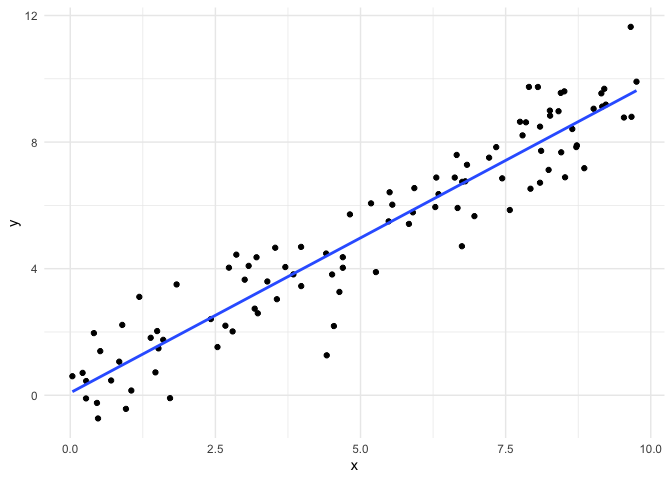
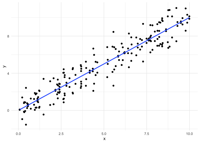
In this example, all of our assumptions are met: the observations are
independent, the relationship between the variables is linear, the error
follows a normal distribution and the error has the same variance for
each observation. Let’s see what the residual plot looks like.
1 | correct_assumptions_lm = lm(y ~ x, data = correct_assumptions) |
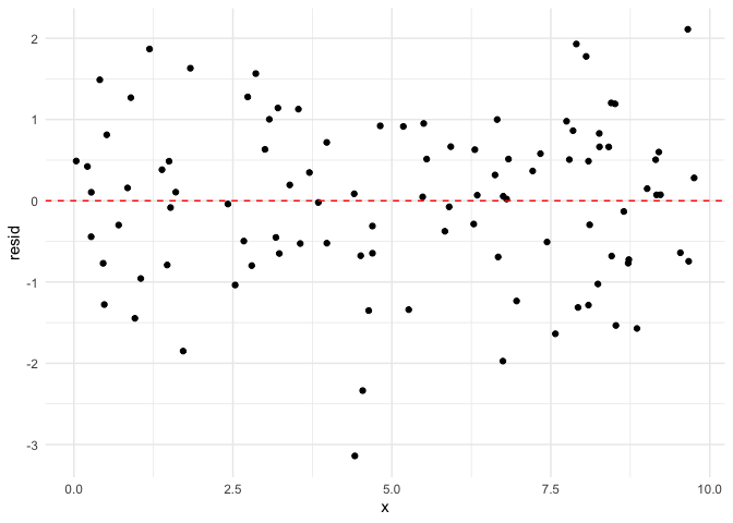
Next, we will demonstrate what residuals look like when these
assumptions are not met.
Equal Variance
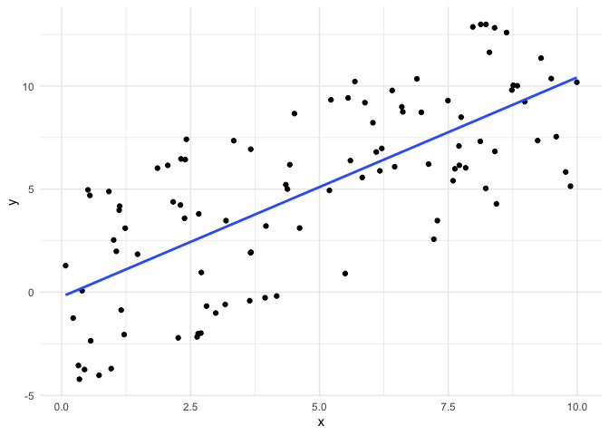
Let’s create some data where the equal variance assumption is violated.
1 | # draw x's uniformally over interval [0, 10] |
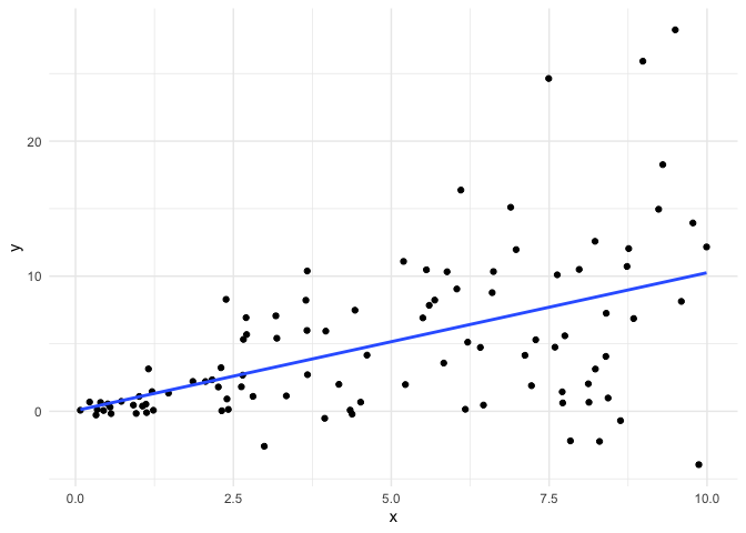
Now, we fit a linear model with this data and look at the residuals.
1 | uneq_var_lm = lm(y ~ x, data = uneq_var) |
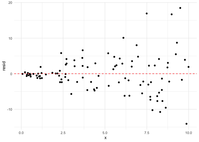
We can clearly see that the residuals around $x=0$ are much less
dispersed than the residuals around $x=10$. When the equal variance
assumption is violated, we typically see a “funnel” shape to the
residuals.
Normal Error
Let’s create some data where the normal error assumption is violated.
1 | # we will use the same x's as before |
Now, we fit a linear model with this data and look at the residuals.
1 | unif_err_lm = lm(y ~ x, data = unif_err) |
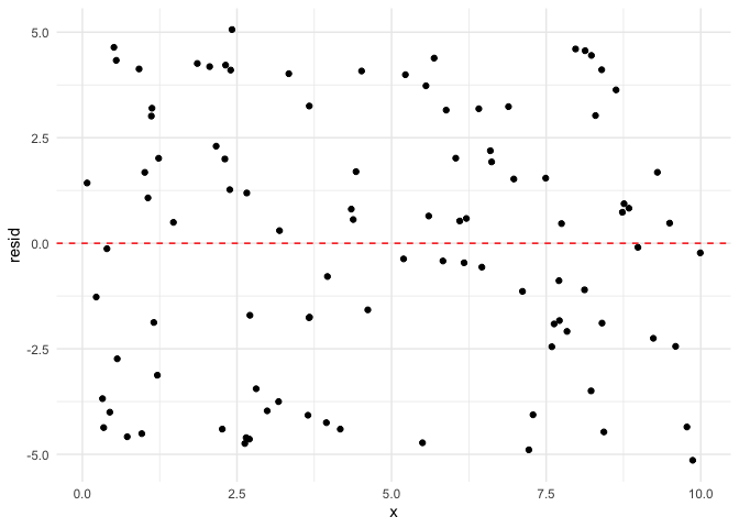
This is what the error looks like with uniform error. Let’s also look at
a more extreme example where we either have error 1 or -1.
1 | # use the same x's as before |

1 | binom_err_lm = lm(y ~ x, data = binom_err) |
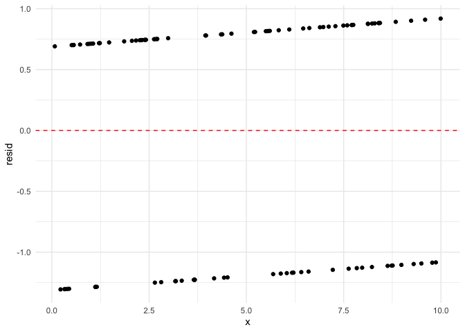
Now we can see the error is definitely not normally distributed. If it
were, there would be more observations close to 0.
Independence
It is not always possible to determine if the independence assumption
isn’t met by looking at residual plots. However, we will show one
example where we can.
1 | # create some normal error |
Now let’s look at the residuals.
1 | dependent_lm = lm(y ~ x, data = dependent) |
Note that the error is symmetrical about zero.
Nonlinearity
Finally, we’ll make some data where the relationship is not linear.
1 | # use the same x's as before |
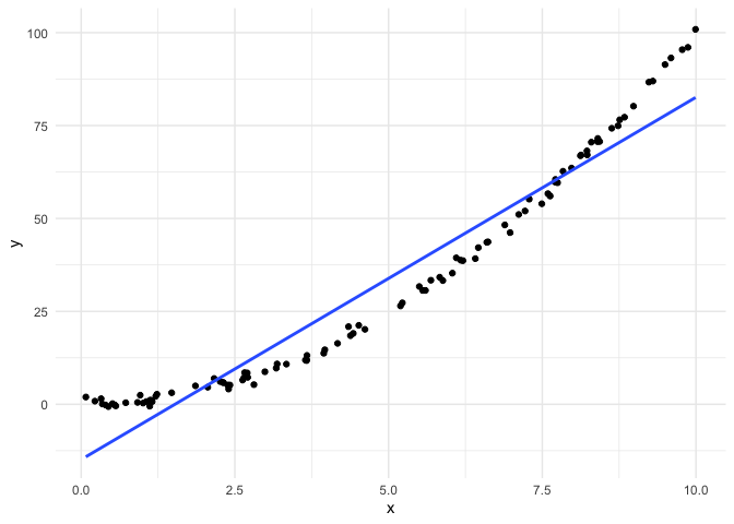
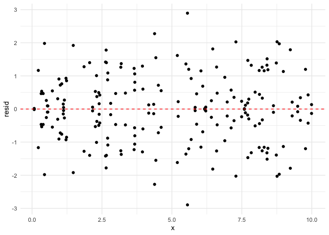
Now let’s look at the residuals.
1 | non_lin_lm = lm(y ~ x, data = non_lin) |
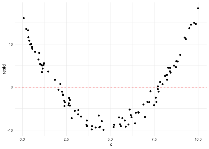
As we can see, the residuals follow a very clear quadratic pattern.